Which Group does a name belong to?

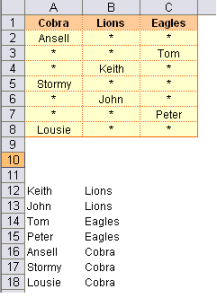
Consider this problem

The table above gives the groups in which each of the members belong. the problem here is to find out in which group one of the member belongs to e.g. Keith (A12). The formula used in B12 is

=INDEX($A$1:$C$1,1,SUMPRODUCT(- –ISNUMBER(SEARCH(A12,$A$2:$C$8)),{1,2,3}*{1;1;1;1;1;1;1}))

The way this works is

• Search function searches for Keith (A12) in the array A2:C8. It returns #VALUE! for cells where Keith is not present and 1 for the cell in which Keith is present
• Isnumber returns True for the cell in which Keith is present and False for the rest
• Operator – – changes True and False to numbers 1 and 0 respectively
• Thus we have an array of 0s and one 1 with 7 rows and 3 columns
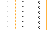
• We now generate an array with {1,2,3}*{1;1;1;1;1;1;1}. This array is of the form

• Sumproduct multiplies the earlier generated array of 0 and 1 with our array such that it returns the column number of cell in which Keith is present – 2 in this case
• Index simply returns the equivalent group from the header array A1:C1 – Lions in this case.

Can you figure out a way of not putting the array manually by using the function row and column functions.

Lookup for “contains”

Here is a method for looking up “contains” from the lookup value array.
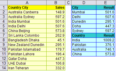
Consider the problem below. I have sales figures for Asia Pacific countries. The lookup value extracted from the system is in the format “Country City”

The expected results are given in the table D1:E11.

Here is the solution using search and sumproduct. You may use array function instead of sumproduct. Suit yourself.

E2=SUMPRODUCT(––ISNUMBER(SEARCH(D2,CountryCity)),Sales)

where, CountryCity is A2:A14 and Sales is B2:B14

You do not need to change the formula while computing for a country figure. The same formula works perfectly.

Now, how does this formula work,

• Search function looks for the lookup city or country in all cells of CountryCity. (You could use Find function but it is case-sensitive). For cells which contains the lookup city or country it returns a number
• Isnumber converts this to True for cells containing the lookup value. Rest are False
• The operator –– converts True to 1 and False to 0 (Refer earlier post)
• Sumproduct multiplies the array of 1’s and 0’s with the Sales array and returns the summation of Sales figure where the “contains” for lookup value is True

Have a great weekend 🙂

Cell value from a grid

While we can use vlookup or hlookup to return a cell value in a particular row or column. Is there a way we can lookup from both row and column to return a particular value from a cell in a grid?

Consider the case below:

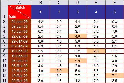
(Yes, I have added more colours to the table this time 🙂 )

The construct is such that every week 5 batches of measurement is carried out. The dates are given in cells A2:A14 and batch numbers are given in cells B1:F1.

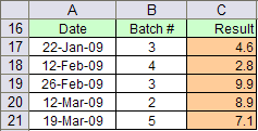
Result table for measurement for specific dates and batches is given in the table below:

You could use one of the following formulas to arrive at the result:

Method1: vlookup with match

C17=VLOOKUP(A17,A2:F14,MATCH(B17,A1:F1,0),FALSE)

Of course, you could find the same result with hlookup with match. Only remember to lookup in a row instead of a column

Method2: Index with match

C18=INDEX(B2:F14,MATCH(A18,A2:A14,0),MATCH(B18,B1:F1,0))

Method3: Indirect with address and match

C19=INDIRECT(ADDRESS(MATCH(A19,A2:A14,0)+ROW(A2)-1,MATCH(B19,B1:F1,0)+COLUMN(B1)-1))

And now the bonus formula – using array

Method4: Sum as an array function

C20 {=SUM(($A$2:$A$14=A20)*($B$1:$F$1=B20)*B2:F14)}

Array formula is entered with ctrl+shift+enter

Method5: Use sumproduct as an alternate for array function

C21=SUMPRODUCT(($A$2:$A$14=A21)*($B$1:$F$1=B21)*B2:F14)

Use one of the above formulas or make one for yourself and share with others. Have fun 🙂

The trick of ––

You read it right. Its going to be a quick post but at the end of it, you would be glad that you read it.

Trick1: Text to Number

 Consider this
=ISNUMBER(LEFT(12345,1)) – this returns FALSE as this simplifies to =ISNUMBER(“1”)

However, =ISNUMBER(––LEFT(12345,1)) returns TRUE. The two minus signs in conjunction “––” converts text “1” to number 1

So, also =––”1″ equals numeric 1

Trick2: Boolean {TRUE, FALSE} to numeric equivalent {1,0}

Consider,

{=SUM({1,2,3,0,5}<>0)} This is an array formula which reduces to

=SUM({TRUE, TRUE, TRUE, FALSE, TRUE}) and returns a 0

However,

{=SUM(––({1,2,3,0,5}<>0))} correctly puts a 1 for every TRUE and 0 for every FALSE and returns a 4

Check this,

Key in =(1=1) – this returns a TRUE

Now =––(1=1) returns a 1

Before you ask, you will not obtain the same result if you replace –– with +

You may keep this in mind and find a use of it someday 🙂

Extracting the nth occurence from an array

In one of the earlier posts, I extracted the first, last, min and max occurence from an array for a particular lookup. Refer this post.

The next step perhaps would be to answer if it is possible to extract the second, third occurences and so on. Consequently to extract all occurences for a particular lookup_value.

Consider the same example, as earlier:

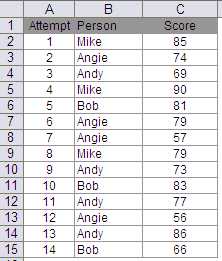
Each of the 4 persons randomly appear for a test and their scores are recorded. I had given methods to extract the scores for 1st and last attempt by each of the 4 perons. Now lets find out their scores for 2nd, 3rd, etc attempts

The table above gives the results. Row 1 gives the number of attempt.

The formula used for getting to the result is

F2=IF(COUNTIF(Person,$E2)>=F$1,INDIRECT(ADDRESS(SUMPRODUCT(LARGE((Person=$E2)*ROW($B$2:$B$15),COUNTIF(Person,$E2)+1-F$1)),3)),”-“)

Person is B2:B15

As you would see, I have used sumproduct to avoid using array formula and a combination of indirect and address to extract results.

Here are the steps to understand this formula –

• Lets begin with the component LARGE((Person=$E2)*ROW($B$2:$B$15),COUNTIF(Person,$E2)+1-F$1
• Remember Large function has the syntax LARGE(array,k) which returns the kth largest value from the array. For example if k=2, then the function returns second largest value in the array.
• Now, (Person=$E2)*ROW($B$2:$B$15) would create an array like {0,2,0,0,5,0,0,0,9,0,0,0,0,0,0} which is essentially the row numbers of cells in the array where Person=Mike is true
• For the k part in large function, I have entered COUNTIF(Person,$E2)+1-F$1. Mike occurs 3 times in array Person, so the k would be 3,2,1, such that 1st attempt score is followed by 2nd attempt score and so on
• Once this is clear, rest is easy
• Address function has syntax Address(row_num, column_num, [abs_num]). row_num is given from the large function, column_num is entered as 3, which is the column number of Score, [abs_num] is omitted which returns address in absolute eg $C$2
• Indirect(“$C$2”) returns the value inC2.
• If condition at the beginning simply evaluates if we have exhausted all occurences of Mike. Once done, it returns a “-“.

§ Note: This also is a better way for multiple extraction because sorting of original table is not required. 

There are 3 other alternative formulas given in the earlier post to achieve the same result.

Else, if one method is sufficient for you, use this and have fun 🙂

Sum – Year to Date

The problem here is summing sales figure from the start of the year to a particular month

Sales of 2 products (Item1 and Item2) is given for an entire year – Jan to Dec. The objective is to find cummulative sales till a particular month. For instance the input is Item1 and Jun – where the output should be sum of sales of Item1 from Jan to Jun (highlighted in yellow).

The desired result is given in the table above. I have used offset function to obtain the result. The function is used with multiple width.

The formula used in C6 is =SUM(OFFSET($A$1,MATCH(B6,$A$2:$A$3,0),1,1,MATCH(A6,$B$1:$M$1,0)))

The first match function returns 1, which is number of rows to offset from the reference A1, the second match function returns 6 – position of month Jun in Jan to Dec – which equals the width of column to sum i.e. Jan to Jun.

Note that this is entered as a simple formula and not an array formula.

The formula can be dragged down to obtain result in C7 –  which is summation of sales of Item2 for YTD Mar.

Thanks Bret for highlighting this problem.

Have fun 🙂

 

First, Last, Min, Max for a particular value in an array

Consider a set-up where 4 users randomly appear for a test. Their scores are recorded in the order in which they appear for the test. Our objective is to find their scores in the first and last attempts and also their minimum and maximum scores. Here are the users and their scores:

The objective is to find the first, last, min and max score for each user. The solution looks like this:

For first attempt score, the formula is a simple vlookup

F2=VLOOKUP(E2,$B$2:$C$15,2,FALSE)

Person is B2:B15 and Score is C2:C15

For max score, the formula is simply:

H2 {=MAX(IF(Person=E2,Score,0))} entered as an array formula with ctrl+shift+enter

Similarly, for min score, the formula is

I2 {=MIN(IF(Person=E2,Score,100))} entered as an array formula with ctrl+shift+enter

I have entered 100 as it is greater than the largest number in Score. You may replace this with max(Score)+1.

Now for last attempt score, you could use one of the 3 sets of formulas

1. Using Index function – array formula

G2 {=INDEX(Score,MAX((Person=E2)*ROW(Person))-ROW(Person)+1)} entered as an array formula with ctrl+shift+enter

In this formula, max function finds out the last row number for a particular user. For instance for user Andy, MAX((Person=E2)*ROW(Person)) returns 14. To return the score for Andy in the last attempt, I have used index function. The minus part of ROW(Person)+1 simply takes care of cells above array Score.

2. Indirect-address function – array formula

G2 {=INDIRECT(ADDRESS(MAX((Person=E2)*ROW(Person)),3))} entered as an array formula with ctrl+shift+enter

If you feel uncomfortable with entering a number in the formula, you could replace 3 with column(Score)

3. Index – Sumproduct function

If you are tired of using array formulas, sumproduct offers some respite

G2=INDEX(Score,SUMPRODUCT(MAX((Person=E2)*ROW(Person)))-ROW(Person)+1)

The formula is similar to the Index with array formula. Here sumproduct is used differently then the normal usage. Notice that there is only one array in sumproduct. The function treats the parameters entered as an array, so we need not enter it as an array formula.

Similarly, indirect address formula can also be entered with sumproduct without entering it as an array formula.

Give it a try. Have fun 🙂

Answer:

DPD analysis using two condition sum

Days past due analysis, two condition sum, bucketing data, frequency function

Here I have carried out a days past due (DPD) analysis. This requires organizing data in various days bucket and makes use of conditional sum function.

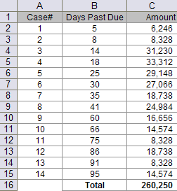
14 cases are presented. Each case has a days past due and a corresponding amount. The objective is to put these numbers in various previously identified buckets

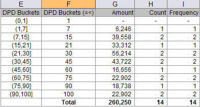
The days past due is defined as (0,1] which means 0<DPD<=1 and so on. This is re-written as in column F.

To calculate the amount in column G the following formulas are used, where DPD is the array B2:B15

G2 {=SUM(IF((DPD>0)*(DPD<=$F2),C$2:C$15,0))}

G3 {=SUM(IF((DPD>$F2)*(DPD<=$F3),C$2:C$15,0))} which can then be dragged till end of column

Both entered as array formula with ctrl+shift+enter

To count occurences in each DPD bucket the following formulas are used

H2 {=SUM(IF((DPD>0)*(DPD<=$F2),1,0))}

H3 {=SUM(IF((DPD>$F2)*(DPD<=$F3),1,0))} which can then be dragged to end of column

You could also use the frequency function for counting occurences

Enter formula in I2 =FREQUENCY(DPD,F2:F11)

Select I2 to I11, press F2 followed by ctrl+shift+enter

Note that the two conditions entered for summing is akin to using SUMIF with criteria as AND(cond1, cond2). However, AND criteria does not work with SUMIF.

Also one could use nested if to achieve the same result. The above format simplifies nested if through using the following logic

TRUE*TRUE=TRUE

All other permutations give a FALSE result, which is exactly a two condition AND criteria.

Have fun figuring this out 😉

Lookup_value as array

lookup_value as array, why lookup over vlookup, multiple lookup_value in single lookup function, sum(lookup)

In one of my earlier posts, I had illustrated passing an array for col_index_num in vlookup. Refer Extract and sum vlookup results.

We now look at the possibility of passing an array for lookup_value in vlookup. Refer the example below:

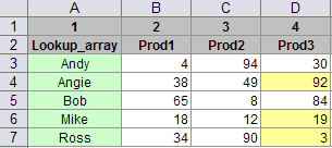
If we were required to sum the sale of Prod3 for Angie, Mike and Ross (cells highlighted in yellow), can we do it through a single vlookup function. Lets say an array is defined as {Ross, Mike, Angie} as salesperson.

This vlookup function

{=SUM(VLOOKUP(salesperson,A3:D7,4,FALSE))} entered as an array with ctrl+shift+enter gives the result as 3 – which corresponds to sale of Prod3 by Ross (first element in the array salesperson). So clearly the array function is not working!

Lets now try the lookup function. Revise the above formula as

{=SUM(LOOKUP(salesperson,A3:D7))}

OR

{=SUM(LOOKUP(salesperson,A3:A7,D3:D7))}

which depends on your comfort with the two syntax for lookup

• LOOKUP(lookup_value,array)
• LOOKUP(lookup_value,lookup_vector,result_vector)

entered as an array formula with ctrl+shift+enter

The formula works and it correctly returns 114

The point to notice here is that lookup_array needs to be in ascending order.

Have fun. This is only the second time that I have used lookup function. It also explains why in the previous post – Text to numbers – method 2, I have used lookup and not vlookup.

Have fun 🙂

Text to Numbers

Just like that, each alphabet corresponds to a number, summing up alphabets

I cant really see how this post could be useful to you. One of my friends who believed in numerology brought this problem to me of converting names to numbers. Here is the solution that we worked out. You may treat this as a Just Like That entry until it finds any use.

Lets say the names are stored in column A, have worked out a numerical equivalent in column B using the equivalence (A or a =1) and (Z or z = 26) with all other alphabets in between

Method 1: Using CODE function

For windows CODE(text) returns the ANSI code of the first character in the text string.

• code(“A”)=65 and code(“Z”)=90 with all other upper case alphabets in between
• code(“a”)=97 and code(“z”)=122 with all other lower case alphabets in between

The formula in B2 {=SUM(CODE(MID(LOWER(A2),ROW(INDIRECT(“1:”&LEN(A2))),1))-96)}

entered as an array formula with ctrl+shift+enter

Here lower function is used so that all alphabets are treated as lower case and ansi code is from 97 to 122

Hence, 96 is subtracted so that a has numerical equivalent of 1

Cell A4 (Anup Agarwal) has space between the first name and last name. We can use substitute function to replace the space with no space. The revised formula in cell B4 is

B4 {=SUM(CODE(MID(LOWER(SUBSTITUTE(A4,” “,””)),ROW(INDIRECT(“1:”&LEN(SUBSTITUTE(A4,” “,””)))),1))-96)}

again entered as an array formula with ctrl+shift+enter

Method 2: Using lookup function

You can avoid using CODE function and use the lookup function to achieve the same result. Have defined the following table as equivalent

 

The formula entered in B2  {=SUM(LOOKUP(MID(A2,ROW(INDIRECT(“1:”&LEN(A2))),1),equivalent))}

entered as an array formula with ctrl+shift+enter

The formula entered in B4 is

{=SUM(LOOKUP(MID(SUBSTITUTE(A4,” “,””),ROW(INDIRECT(“1:”&LEN(SUBSTITUTE(A4,” “,””)))),1),equivalent))}

entered as an array formula with ctrl+shift+enter

Have fun and let me know if you ever find use of it 🙂