Cell value from a grid

While we can use vlookup or hlookup to return a cell value in a particular row or column. Is there a way we can lookup from both row and column to return a particular value from a cell in a grid?

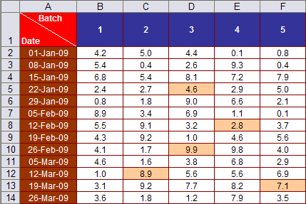
Consider the case below:

(Yes, I have added more colours to the table this time 🙂 )

The construct is such that every week 5 batches of measurement is carried out. The dates are given in cells A2:A14 and batch numbers are given in cells B1:F1.

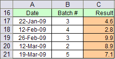
Result table for measurement for specific dates and batches is given in the table below:

You could use one of the following formulas to arrive at the result:

Method1: vlookup with match

C17=VLOOKUP(A17,A2:F14,MATCH(B17,A1:F1,0),FALSE)

Of course, you could find the same result with hlookup with match. Only remember to lookup in a row instead of a column

Method2: Index with match

C18=INDEX(B2:F14,MATCH(A18,A2:A14,0),MATCH(B18,B1:F1,0))

Method3: Indirect with address and match

C19=INDIRECT(ADDRESS(MATCH(A19,A2:A14,0)+ROW(A2)-1,MATCH(B19,B1:F1,0)+COLUMN(B1)-1))

And now the bonus formula – using array

Method4: Sum as an array function

C20 {=SUM(($A$2:$A$14=A20)*($B$1:$F$1=B20)*B2:F14)}

Array formula is entered with ctrl+shift+enter

Method5: Use sumproduct as an alternate for array function

C21=SUMPRODUCT(($A$2:$A$14=A21)*($B$1:$F$1=B21)*B2:F14)

Use one of the above formulas or make one for yourself and share with others. Have fun 🙂

Read Full Post »

Vlookup – col_index_num

A quick trick for people who often use vlookup.

Often when the table array is large, calculating the col_index_num can be quite a hassle. Here is an easy way to do this

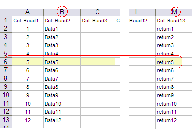
Lets say our table array is B1:M13 and we want vlookup to return result from the last column (column M), here’s how we can do this

Say lookup_value is Data5, we would need to key in this formula

=VLOOKUP(B6,B2:M13,(COLUMN(M1)-COLUMN(B1))+1,FALSE)

col_index_num here is (COLUMN(M1)-COLUMN(B1))+1

The formula correctly gives the result return5

Hope you find this useful 🙂

Read Full Post »

Unraveling a table

Here is the problem that I faced

 

 

 

 

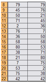
I had to extract the entries in the table row-wise and populate this in a single column.
Here is one way of doing this:

• Enter A8=OFFSET($A$2,INT((ROW()-ROW($B$8))/5),MOD((ROW()-ROW$B$8)),5),1,1)
• Drag down till the entire table is unravelled.

What if we had to unravel the table column wise i.e. in the order A2, A3, A4 etc

Here is the formula that you need to enter in B8 and drag till the last table entry

B8=OFFSET($A$2,MOD((ROW()-ROW($B$8)),3),INT((ROW()-ROW($B$8))/3),1,1)

One could also extract the table in a columnar format. We would have to switch row for column to do so.

mod has the syntax mod(number, divisor) and returns the remainder when number is divided by the divisor. In the above case when the divisor is 3, it returns 0,1,2,01,2 and so on

int(number) returns the nearest integer less than or equal to the number. In the above case int returns 0,0,0,1,1,1,2,2,2 and so on

This is exactly what we need to offset from the reference in the table and unravel it.

Note the divisor in the two formulas, in the first formula the divisor is 5, which is equal to number of columns in the table

In the second formula divisor is 3, which is equal to number of rows in the table

This could also be computed through columns(A2:E4) and rows(A2:E4) respectively

Let me know if you ever find this tip useful or are not clear about any part of the post.

In the meantime, have fun working with excel 🙂

Read Full Post »

Generating a series of numbers

In some of my earlier posts, I have manually populated some cells with a series of numbers (numbers 1-4 were manually populated in the post multiple extraction through vlookup). Here is a way we can do away with this by using functions row() and column()

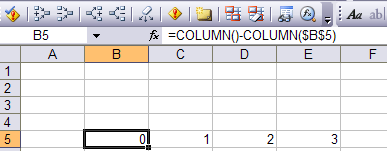
Lets say you want to populate 0 to 10 in a column in cells B5 through L5:
Enter B5=COLUMN()-COLUMN($B$5)

On dragging upto L5, it populates the cells with the series 0 – 10.

As you can figure out

• column() returns the column number of that particular cell
• If a reference is provided [eg. column(B5)] – it returns the column number of the referred cell – 2 in the above example

If we were to populate numbers in a row, the function row() could have been used. To populate cells A1 to A11 with numbers 0 to 10,

• A1 = row()-row($A$1) – drag till cell A11

’tis done!

§ I am going to leave an example for you to think about the utility of this. Also would use this function in my next post.

√ To sum first 10 natural numbers – 1 to 10 i.e Σ(1,2..10)

Enter this in any cell =SUM(ROW(A1:A10)) as an array formula i.e. ctrl+shift+enter instead of enter. This gives the result as 55

The formula is interpreted as SUM({1;2;3;4;5;6;7;8;9;10})

If you found this interesting or would like some more help on this, let me know 🙂

Read Full Post »

Multiple extraction through vlookup

The problem here is extraction of multiple results from a two column array through a vlookup

 

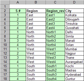
The data available is given in columns B and D. The 4 regions along with their major cities are known. The data needs to be arranged as in the table below

Start by sorting on region (column B)

Column A is populated with serial numbers such that each region has a fresh series

Cell A3=1, Cell A4=IF(B4=B3,A3+1,1) – drag till end of column

Column C is concatenation of columns B and A

Cell C3=CONCATENATE(B3,A3) – drag till end of column

This enables us to have a one on one mapping with region and cities

Now, to generate the result table on the right

Cells – G1:J1 is manually populated with numbers 1 through 4

Cell G2=VLOOKUP(CONCATENATE($F2,G$1),$C$3:$D$18,2,FALSE) – drag till end of column and end of row

’tis done!

Alternative solution 1 using offset

To generate the table in F11:G14

Populate F11 to F14 with East, West, North, South

Here again, we would have to sort on region (column B) first

Enter G11 = IF((COLUMN()-COLUMN($G$1))<COUNTIF($B$3:$B$18,$F11),OFFSET($D$3,MATCH($F11,$B$3:$B$18,0)-1+(COLUMN()-COLUMN($G$1)),0,1,1),””)

Here,

column()-column($G$1) generates numbers 0,1 etc

countif – returns number of occurences of east, west, etc

offset – offsets from the reference cell D3, number of rows given by first occurence of east – provided by match function + serial number given by the column function

You could seperate each of the functions to understand how this works. If you need any help in understanding do let me know

 

Drag to the right and below to populate the entire table

’tis done again

Alternative solution 2 using index

To generate the table in F18:G21

Populate F18 to G21 with East, West, North, South

Enter G18 =IF((COLUMN()-COLUMN($G$1))<COUNTIF($B$3:$B$18,$F11),INDEX($D$3:$D$18,MATCH($F11,$B$3:$B$18,0)+(COLUMN()-COLUMN($G$1))))

Drag to the right and down to populate the entire table.

’tis done once again

Read Full Post »