Feeds:
Posts
Comments

Posts Tagged ‘Conditional formatting’

To track status of a project or tasks, RAG (Red, Amber, Green) report is commonly used. Given below is a sample RAG report as on 04-Jun-09

tip26-RAG_report

The following logic is used for creating the report
 

For Open tasks: 

  • Red: SCD – today()+1 is -ve
  • Amber: SCD – today()+1 is 0
  • Green: SCD – today()+1 is +ve

For Closed tasks:

  • Red: SCD – ACD+1 is -ve
  • Amber: SCD – ACD+1 is 0
  • Green: SCD – ACD+1 is +ve

SCD = Scheduled Completion Date

ACD = Actual Completion Date

The following formulas are used
C2=CHOOSE(WEEKDAY(B2),”Sun”,”Mon”,”Tue”,”Wed”,”Thu”,”Fri”,”Sat”)

H2=IF(F2=”Open”,CHOOSE(2+SIGN(E2-TODAY()+1),”Red”,”Amber”,”Green”),CHOOSE(2+SIGN(E2-G2+1),”Red”,”Amber”,”Green”))

Column H is conditionally formatted to colour the cells –  Red, Amber or Green
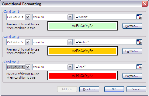
tip26-RAG_report1

Choose function Uses index_num to return a value from the list of value arguments has the syntax CHOOSE(index_num,value1,value2,…)

Sign function returns (0,+1,-1) depending on whether the input is 0,+ve or -ve

You could change the formula depending on the logic you want to use for RAG.

Have fun 🙂

Read Full Post »

Here is a list of 10 formatting tips that would help make your excel worksheet look great

  1. Toggle grid – After you have done your analysis, make the gridlines disappear from your worksheet. It gives a much cleaner look and is very eye friendly. Here is how you do it – Add Form toolbar – View > Toolbars > Forms and click on Toggle Grid Grid-Toggle
  2.  

  3. Highlight through conditional formatting – use conditional formatting to add colours to cells that you wish to highlight. It is easier to find something that you are looking for if it is coloured. Here is an example of highlighting errors in an array.
    tip24-highlight
    Format all other cells in the array with the format painter brush format-painterto highlight all errors in the array
  4.  

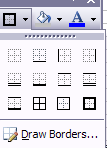
  5. Add cell borders – if there are certain cells that you wish to highlight, for instance cells with array summations, use cell borders. You would find this in formatting toolbar tip24-add-border
  6.  

  7. Table grids of different colours – the default colour for all borders is black. Use colours to your advantage and change it from Format > Cells…>Border>Color:
  8.  

  9. Maintain consistent format -Unless the analysis specific requires it, you may like to maintain consistent format for numbers –
      √ Have same number of decimal places – use increase/decrease decimal on formatting toolbar
      √ Date in same format – choose a format from Format > Cells > Number > Date. Once chose you could use the format painter brush to apply to all cells with dates in them
  10.  

  11. Resize cells – Resize cells according to the content. Resize-cells Excel can automatically resize cells according to the contents of the cell. In this example, take the cursor on the line between D and E. Double click when a cross hair appears
  12.  

  13. Avoid cell merge as far as possible – Resize cells, insert columns but avoid cell merge as they become messy after some time and are difficult to handle
  14.  

  15. Wrap text – If there is too much data in a cell, consider wrapping the text. Format > Cells…>Alignment>Wrap text
  16.  

  17. Printing with gridlines – Even if toggle grid is on, print of the worksheet may not display the grids. To display grids – File > Print > Preview > Setup… > Sheet > Gridlines
  18.  

  19. To hide errors in printsFile > Print > Preview > Setup… > Sheet > Cell errors as: <blank>

Have fun formatting worksheets 🙂

Read Full Post »

Here is how you can play the game Cows and Bulls in excel

The objective of the game is to guess the secret number (which is hidden from the player). The player can guess the number as many times. If the matching digits are on their right positions, they are “bulls”, if on different positions, they are “cows”. Example given below

tip17-cowsnbulls

The formula for cows:
C3 {=COUNT(MATCH(MID(B3,ROW($1:$4),1),MID($B$1,ROW($1:$4),1),0))}
(entered as an array formula, ctrl+shift+enter)

The formula for bulls
D3 {=SUM(IF(MID($B$1,ROW($1:$4),1)=MID(B3,ROW($1:$4),1),1,0))}
(entered as an array formula, ctrl+shift+enter)

Drag the formula down. You could keep entering your guesses in column B

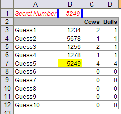
One could also highlight the cell if the number is guessed correctly, through conditional formatting
Click B3 and through Format>Conditional Formatting…
tip17-cowsnbulls-frmtng
Copy the format to all cells in column B through Format Painter format-painter brush on the toolbar

Tip: If you are playing the game alone and have no one to give you a 4 digit number, you could use rand() function

In the secret number cell enter = ROUND(RAND()*10^4,0), Press F2 and F9 – this would freeze the random number. Make sure that no digits are repeated and the random number is 4 digits long. You can use len function and check duplicate function for that

Have fun playing the game 🙂

Read Full Post »

Tips for identifying duplicates in a list

Lets say the list is

Tip#1: Conditional formatting
Go to conditional formatting box and enter
“Formula is” =COUNTIF($A$1:$A$8,A1)>1
Format the box with a different colour (yellow in above)
Format paint for all cells A1 to A8 with ‘format painter’ brush

Tip#2: Array formula
Enter an array formula
{=IF(MAX(COUNTIF(A1:A8,A1:A8))>1,”Duplicates”,”No Dups”)}
Array formulas are entered by ctrl+shift+enter
In this example, formula gives result as Duplicates

Tip#3: Flag
In cell B1 enter
=IF(COUNTIF($A$1:$A$8,A1)>1,”Dup”,”No_dup”)
Drag the formula to B8
This flags off the dup entries

Tip#4: create an array of unique entries

Select A1:A8, click Data -> Filter -> Advanced Filter… ->Unique records only

This list is without any duplicates

Read Full Post »