The trick of ––

You read it right. Its going to be a quick post but at the end of it, you would be glad that you read it.

Trick1: Text to Number

 Consider this
=ISNUMBER(LEFT(12345,1)) – this returns FALSE as this simplifies to =ISNUMBER(“1”)

However, =ISNUMBER(––LEFT(12345,1)) returns TRUE. The two minus signs in conjunction “––” converts text “1” to number 1

So, also =––”1″ equals numeric 1

Trick2: Boolean {TRUE, FALSE} to numeric equivalent {1,0}

Consider,

{=SUM({1,2,3,0,5}<>0)} This is an array formula which reduces to

=SUM({TRUE, TRUE, TRUE, FALSE, TRUE}) and returns a 0

However,

{=SUM(––({1,2,3,0,5}<>0))} correctly puts a 1 for every TRUE and 0 for every FALSE and returns a 4

Check this,

Key in =(1=1) – this returns a TRUE

Now =––(1=1) returns a 1

Before you ask, you will not obtain the same result if you replace –– with +

You may keep this in mind and find a use of it someday 🙂

Read Full Post »

Adding errors, texts, numbers, blanks in a list

A quick post.

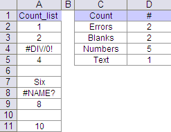
Here is how you can you can count errors, blanks, numbers, texts in a list.

List A2:A11 is defined as Count_list

To count

• Errors       {=SUM(IF(ISERROR(Count_list),1,0))}
• Blanks       {=SUM(IF(ISBLANK(Count_list),1,0))}
• Numbers {=SUM(IF(ISNUMBER(Count_list),1,0))}
• Text           {=SUM(IF(ISTEXT(Count_list),1,0))}

The formulas are entered as array formuals with ctrl+shift+enter

Read Full Post »

Vlookup – col_index_num

A quick trick for people who often use vlookup.

Often when the table array is large, calculating the col_index_num can be quite a hassle. Here is an easy way to do this

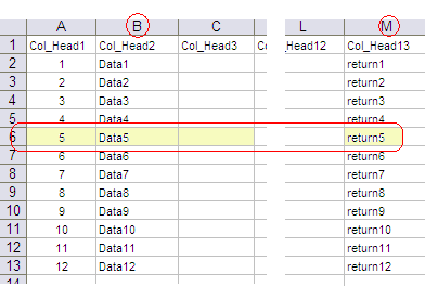
Lets say our table array is B1:M13 and we want vlookup to return result from the last column (column M), here’s how we can do this

Say lookup_value is Data5, we would need to key in this formula

=VLOOKUP(B6,B2:M13,(COLUMN(M1)-COLUMN(B1))+1,FALSE)

col_index_num here is (COLUMN(M1)-COLUMN(B1))+1

The formula correctly gives the result return5

Hope you find this useful 🙂

Read Full Post »