Converting numbers to words

How do we convert numbers to words. Especially useful if you are writing cheques (checks) through printing through a soft file.

The logic given below is one for India – it uses crores and lacs. The logic works for all numbers between 1 and 99,99,99,999 (100 crore -1)

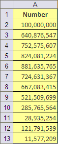
Say the numbers that need to be converted to words are given in column A

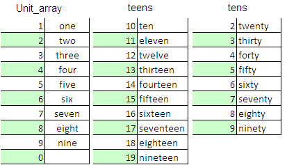
Step 1: Start with defining the following arrays

Step2: Extract units, tens, hundreds, thousands, lacs and crores from the numbers in column A

The result is given Array1 below:

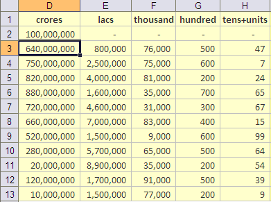
The formulas used are:

For crores: D2=ROUNDDOWN($A2,-7)

For lacs: E2=ROUNDDOWN($A2,-5)-$D2

For thousands: F2=ROUNDDOWN($A2,-3)-SUM($D2:E2)

For hundreds: G2=ROUNDDOWN($A2,-2)-SUM($D2:F2)

For tens & units: H2=$A2-SUM($D2:G2)

Drag till end of columns

Modify the Array1 so that resuts appear as this in Array2:

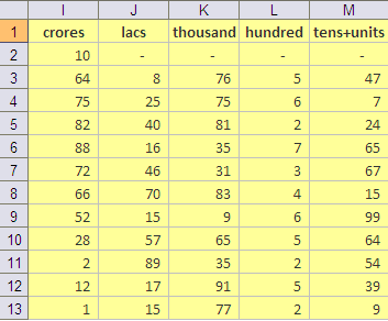
The formulas used are:

For crores: I2=D2/10^7

For lacs: J2=E2/10^5

For thousands: K2=F2/10^3

For hundreds: L2=G2/10^2

For tens+units: M2=H2

Step 3: Convert numbers to words for each column

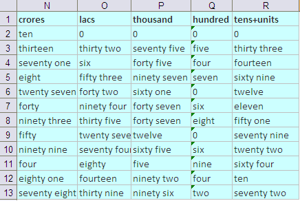
The formulas used are:

Crores: N2=IF(LEN(I2)=1,VLOOKUP(I2,Unit_array,2,FALSE),IF(VALUE(LEFT(I2,1))=1,VLOOKUP(I2,teens,2,FALSE),CONCATENATE(VLOOKUP(VALUE(LEFT(I2,1)),tens,2,FALSE),” “,VLOOKUP(VALUE(RIGHT(I2,1)),Unit_array,2,FALSE))))

Lacs: O2=IF(LEN(J2)=1,VLOOKUP(J2,Unit_array,2,FALSE),IF(VALUE(LEFT(J2,1))=1,VLOOKUP(J2,teens,2,FALSE),CONCATENATE(VLOOKUP(VALUE(LEFT(J2,1)),tens,2,FALSE),” “,VLOOKUP(VALUE(RIGHT(J2,1)),Unit_array,2,FALSE))))

Thousands: P2=IF(LEN(K2)=1,VLOOKUP(K2,Unit_array,2,FALSE),IF(VALUE(LEFT(K2,1))=1,VLOOKUP(K2,teens,2,FALSE),CONCATENATE(VLOOKUP(VALUE(LEFT(K2,1)),tens,2,FALSE),” “,VLOOKUP(VALUE(RIGHT(K2,1)),Unit_array,2,FALSE))))

Hundreds: Q2=VLOOKUP(L2,Unit_array,2,FALSE)

Tens&Units: R2=IF(LEN(M2)=1,VLOOKUP(M2,Unit_array,2,FALSE),IF(VALUE(LEFT(M2,1))=1,VLOOKUP(M2,teens,2,FALSE),CONCATENATE(VLOOKUP(VALUE(LEFT(M2,1)),tens,2,FALSE),” “,VLOOKUP(VALUE(RIGHT(M2,1)),Unit_array,2,FALSE))))

Formula for crores, lacs, thousands, tens&units are similar in logic and construct

The logic used is

• If number is of 1 digit (0 to 9)- then lookup value from Unit_array
• If number starts with 1 (10 to 19) – then lookup value from teens
• For all else (20 to 99) – lookup left digit from tens and right digit from Unit_array and concatenate

Formula for hundreds is simple – lookup value from Unit_array as hundreds can only be from 0 to 9

Step 4: Now the fun part – putting it all together

The formula is simply

B2=PROPER(CONCATENATE(IF(I2>0,N2&” crores “,””),IF(J2>0,O2&” lacs “,””),IF(K2>0,P2&” thousand “,””),IF(L2>0,Q2&” hundred “,””),IF(R2>0,R2,””)))

Have added proper to capitalize the first letters of all words in the text string.

Let me know if it helps you 🙂

Read Full Post »

Multiple extraction through vlookup

The problem here is extraction of multiple results from a two column array through a vlookup

 

The data available is given in columns B and D. The 4 regions along with their major cities are known. The data needs to be arranged as in the table below

Start by sorting on region (column B)

Column A is populated with serial numbers such that each region has a fresh series

Cell A3=1, Cell A4=IF(B4=B3,A3+1,1) – drag till end of column

Column C is concatenation of columns B and A

Cell C3=CONCATENATE(B3,A3) – drag till end of column

This enables us to have a one on one mapping with region and cities

Now, to generate the result table on the right

Cells – G1:J1 is manually populated with numbers 1 through 4

Cell G2=VLOOKUP(CONCATENATE($F2,G$1),$C$3:$D$18,2,FALSE) – drag till end of column and end of row

’tis done!

Alternative solution 1 using offset

To generate the table in F11:G14

Populate F11 to F14 with East, West, North, South

Here again, we would have to sort on region (column B) first

Enter G11 = IF((COLUMN()-COLUMN($G$1))<COUNTIF($B$3:$B$18,$F11),OFFSET($D$3,MATCH($F11,$B$3:$B$18,0)-1+(COLUMN()-COLUMN($G$1)),0,1,1),””)

Here,

column()-column($G$1) generates numbers 0,1 etc

countif – returns number of occurences of east, west, etc

offset – offsets from the reference cell D3, number of rows given by first occurence of east – provided by match function + serial number given by the column function

You could seperate each of the functions to understand how this works. If you need any help in understanding do let me know

 

Drag to the right and below to populate the entire table

’tis done again

Alternative solution 2 using index

To generate the table in F18:G21

Populate F18 to G21 with East, West, North, South

Enter G18 =IF((COLUMN()-COLUMN($G$1))<COUNTIF($B$3:$B$18,$F11),INDEX($D$3:$D$18,MATCH($F11,$B$3:$B$18,0)+(COLUMN()-COLUMN($G$1))))

Drag to the right and down to populate the entire table.

’tis done once again

Read Full Post »