First, Last, Min, Max for a particular value in an array

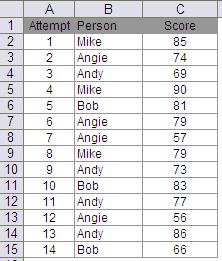
Consider a set-up where 4 users randomly appear for a test. Their scores are recorded in the order in which they appear for the test. Our objective is to find their scores in the first and last attempts and also their minimum and maximum scores. Here are the users and their scores:

The objective is to find the first, last, min and max score for each user. The solution looks like this:

For first attempt score, the formula is a simple vlookup

F2=VLOOKUP(E2,$B$2:$C$15,2,FALSE)

Person is B2:B15 and Score is C2:C15

For max score, the formula is simply:

H2 {=MAX(IF(Person=E2,Score,0))} entered as an array formula with ctrl+shift+enter

Similarly, for min score, the formula is

I2 {=MIN(IF(Person=E2,Score,100))} entered as an array formula with ctrl+shift+enter

I have entered 100 as it is greater than the largest number in Score. You may replace this with max(Score)+1.

Now for last attempt score, you could use one of the 3 sets of formulas

1. Using Index function – array formula

G2 {=INDEX(Score,MAX((Person=E2)*ROW(Person))-ROW(Person)+1)} entered as an array formula with ctrl+shift+enter

In this formula, max function finds out the last row number for a particular user. For instance for user Andy, MAX((Person=E2)*ROW(Person)) returns 14. To return the score for Andy in the last attempt, I have used index function. The minus part of ROW(Person)+1 simply takes care of cells above array Score.

2. Indirect-address function – array formula

G2 {=INDIRECT(ADDRESS(MAX((Person=E2)*ROW(Person)),3))} entered as an array formula with ctrl+shift+enter

If you feel uncomfortable with entering a number in the formula, you could replace 3 with column(Score)

3. Index – Sumproduct function

If you are tired of using array formulas, sumproduct offers some respite

G2=INDEX(Score,SUMPRODUCT(MAX((Person=E2)*ROW(Person)))-ROW(Person)+1)

The formula is similar to the Index with array formula. Here sumproduct is used differently then the normal usage. Notice that there is only one array in sumproduct. The function treats the parameters entered as an array, so we need not enter it as an array formula.

Similarly, indirect address formula can also be entered with sumproduct without entering it as an array formula.

Give it a try. Have fun 🙂

Answer:

Read Full Post »

Identifying duplicates in a list

Tips for identifying duplicates in a list

Lets say the list is

Tip#1: Conditional formatting
Go to conditional formatting box and enter
“Formula is” =COUNTIF($A$1:$A$8,A1)>1
Format the box with a different colour (yellow in above)
Format paint for all cells A1 to A8 with ‘format painter’ brush

Tip#2: Array formula
Enter an array formula
{=IF(MAX(COUNTIF(A1:A8,A1:A8))>1,”Duplicates”,”No Dups”)}
Array formulas are entered by ctrl+shift+enter
In this example, formula gives result as Duplicates

Tip#3: Flag
In cell B1 enter
=IF(COUNTIF($A$1:$A$8,A1)>1,”Dup”,”No_dup”)
Drag the formula to B8
This flags off the dup entries

Tip#4: create an array of unique entries

Select A1:A8, click Data -> Filter -> Advanced Filter… ->Unique records only

This list is without any duplicates

Read Full Post »