Extracting the nth occurence from an array

In one of the earlier posts, I extracted the first, last, min and max occurence from an array for a particular lookup. Refer this post.

The next step perhaps would be to answer if it is possible to extract the second, third occurences and so on. Consequently to extract all occurences for a particular lookup_value.

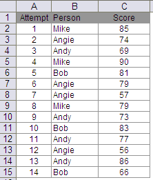
Consider the same example, as earlier:

Each of the 4 persons randomly appear for a test and their scores are recorded. I had given methods to extract the scores for 1st and last attempt by each of the 4 perons. Now lets find out their scores for 2nd, 3rd, etc attempts

The table above gives the results. Row 1 gives the number of attempt.

The formula used for getting to the result is

F2=IF(COUNTIF(Person,$E2)>=F$1,INDIRECT(ADDRESS(SUMPRODUCT(LARGE((Person=$E2)*ROW($B$2:$B$15),COUNTIF(Person,$E2)+1-F$1)),3)),”-“)

Person is B2:B15

As you would see, I have used sumproduct to avoid using array formula and a combination of indirect and address to extract results.

Here are the steps to understand this formula –

• Lets begin with the component LARGE((Person=$E2)*ROW($B$2:$B$15),COUNTIF(Person,$E2)+1-F$1
• Remember Large function has the syntax LARGE(array,k) which returns the kth largest value from the array. For example if k=2, then the function returns second largest value in the array.
• Now, (Person=$E2)*ROW($B$2:$B$15) would create an array like {0,2,0,0,5,0,0,0,9,0,0,0,0,0,0} which is essentially the row numbers of cells in the array where Person=Mike is true
• For the k part in large function, I have entered COUNTIF(Person,$E2)+1-F$1. Mike occurs 3 times in array Person, so the k would be 3,2,1, such that 1st attempt score is followed by 2nd attempt score and so on
• Once this is clear, rest is easy
• Address function has syntax Address(row_num, column_num, [abs_num]). row_num is given from the large function, column_num is entered as 3, which is the column number of Score, [abs_num] is omitted which returns address in absolute eg $C$2
• Indirect(“$C$2”) returns the value inC2.
• If condition at the beginning simply evaluates if we have exhausted all occurences of Mike. Once done, it returns a “-“.

§ Note: This also is a better way for multiple extraction because sorting of original table is not required. 

There are 3 other alternative formulas given in the earlier post to achieve the same result.

Else, if one method is sufficient for you, use this and have fun 🙂

Read Full Post »

Multiple extraction through vlookup

The problem here is extraction of multiple results from a two column array through a vlookup

 

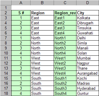
The data available is given in columns B and D. The 4 regions along with their major cities are known. The data needs to be arranged as in the table below

Start by sorting on region (column B)

Column A is populated with serial numbers such that each region has a fresh series

Cell A3=1, Cell A4=IF(B4=B3,A3+1,1) – drag till end of column

Column C is concatenation of columns B and A

Cell C3=CONCATENATE(B3,A3) – drag till end of column

This enables us to have a one on one mapping with region and cities

Now, to generate the result table on the right

Cells – G1:J1 is manually populated with numbers 1 through 4

Cell G2=VLOOKUP(CONCATENATE($F2,G$1),$C$3:$D$18,2,FALSE) – drag till end of column and end of row

’tis done!

Alternative solution 1 using offset

To generate the table in F11:G14

Populate F11 to F14 with East, West, North, South

Here again, we would have to sort on region (column B) first

Enter G11 = IF((COLUMN()-COLUMN($G$1))<COUNTIF($B$3:$B$18,$F11),OFFSET($D$3,MATCH($F11,$B$3:$B$18,0)-1+(COLUMN()-COLUMN($G$1)),0,1,1),””)

Here,

column()-column($G$1) generates numbers 0,1 etc

countif – returns number of occurences of east, west, etc

offset – offsets from the reference cell D3, number of rows given by first occurence of east – provided by match function + serial number given by the column function

You could seperate each of the functions to understand how this works. If you need any help in understanding do let me know

 

Drag to the right and below to populate the entire table

’tis done again

Alternative solution 2 using index

To generate the table in F18:G21

Populate F18 to G21 with East, West, North, South

Enter G18 =IF((COLUMN()-COLUMN($G$1))<COUNTIF($B$3:$B$18,$F11),INDEX($D$3:$D$18,MATCH($F11,$B$3:$B$18,0)+(COLUMN()-COLUMN($G$1))))

Drag to the right and down to populate the entire table.

’tis done once again

Read Full Post »

Identifying duplicates in a list

Tips for identifying duplicates in a list

Lets say the list is

Tip#1: Conditional formatting
Go to conditional formatting box and enter
“Formula is” =COUNTIF($A$1:$A$8,A1)>1
Format the box with a different colour (yellow in above)
Format paint for all cells A1 to A8 with ‘format painter’ brush

Tip#2: Array formula
Enter an array formula
{=IF(MAX(COUNTIF(A1:A8,A1:A8))>1,”Duplicates”,”No Dups”)}
Array formulas are entered by ctrl+shift+enter
In this example, formula gives result as Duplicates

Tip#3: Flag
In cell B1 enter
=IF(COUNTIF($A$1:$A$8,A1)>1,”Dup”,”No_dup”)
Drag the formula to B8
This flags off the dup entries

Tip#4: create an array of unique entries

Select A1:A8, click Data -> Filter -> Advanced Filter… ->Unique records only

This list is without any duplicates

Read Full Post »