Insert spaces – revisited

I had earlier posted a solution on inserting spaces between continuous cells in a list. Though the solution works fine for a few items (46 items in the earlier example), it returns a blank for items after that. The solution had comprised of using the formula C1+1/3; where C1=1 and dragging it so that two fractional numbers are inserted between the integers i.e. 1, 1¹⁄3, 1²/3, 2 and so on. Excel processes these as recurring decimals and possibly rounds off recurring decimals. So the rounding off errors gets added up to the point where it is large enough for indirect function to fail.

Have a look at this

 

 

 

 

Where F2=INDIRECT(“A”&E2)

The indirect formula continues to work as long as the error ε<1E-15. Any bigger error returns a function error.

Have solved this problem through using a combination of int and mod, which works well for very large lists as well

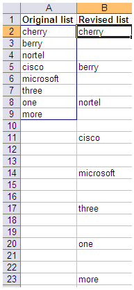
The original list is given in array A2:A9 (which has also been defined as Original_list).

Enter B2=IF(MOD((ROW()-ROW($B$2)),3)=0,INDEX(Original_list,INT((ROW()-ROW($B$2))/3)+1),””)

Drag till the entire list is mapped

You could change the constant 3 to a higher number if you need to insert more spaces between the entries

Let me know if you find this useful 🙂

Read Full Post »

Unraveling a table

Here is the problem that I faced

 

 

 

 

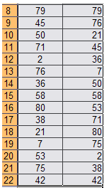
I had to extract the entries in the table row-wise and populate this in a single column.
Here is one way of doing this:

• Enter A8=OFFSET($A$2,INT((ROW()-ROW($B$8))/5),MOD((ROW()-ROW$B$8)),5),1,1)
• Drag down till the entire table is unravelled.

What if we had to unravel the table column wise i.e. in the order A2, A3, A4 etc

Here is the formula that you need to enter in B8 and drag till the last table entry

B8=OFFSET($A$2,MOD((ROW()-ROW($B$8)),3),INT((ROW()-ROW($B$8))/3),1,1)

One could also extract the table in a columnar format. We would have to switch row for column to do so.

mod has the syntax mod(number, divisor) and returns the remainder when number is divided by the divisor. In the above case when the divisor is 3, it returns 0,1,2,01,2 and so on

int(number) returns the nearest integer less than or equal to the number. In the above case int returns 0,0,0,1,1,1,2,2,2 and so on

This is exactly what we need to offset from the reference in the table and unravel it.

Note the divisor in the two formulas, in the first formula the divisor is 5, which is equal to number of columns in the table

In the second formula divisor is 3, which is equal to number of rows in the table

This could also be computed through columns(A2:E4) and rows(A2:E4) respectively

Let me know if you ever find this tip useful or are not clear about any part of the post.

In the meantime, have fun working with excel 🙂

Read Full Post »