Sum – Year to Date

The problem here is summing sales figure from the start of the year to a particular month

Sales of 2 products (Item1 and Item2) is given for an entire year – Jan to Dec. The objective is to find cummulative sales till a particular month. For instance the input is Item1 and Jun – where the output should be sum of sales of Item1 from Jan to Jun (highlighted in yellow).

The desired result is given in the table above. I have used offset function to obtain the result. The function is used with multiple width.

The formula used in C6 is =SUM(OFFSET($A$1,MATCH(B6,$A$2:$A$3,0),1,1,MATCH(A6,$B$1:$M$1,0)))

The first match function returns 1, which is number of rows to offset from the reference A1, the second match function returns 6 – position of month Jun in Jan to Dec – which equals the width of column to sum i.e. Jan to Jun.

Note that this is entered as a simple formula and not an array formula.

The formula can be dragged down to obtain result in C7 –  which is summation of sales of Item2 for YTD Mar.

Thanks Bret for highlighting this problem.

Have fun 🙂

 

Read Full Post »

Evaluating step functions

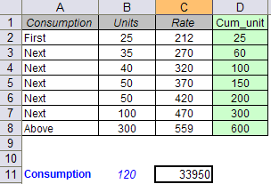
This problem is on step functions. Certain utility company charges me in this manner

For the first 25 units of consumption, the rate is 212 per unit, for next 35 units, the rate is 270 per unit and so on.

I have calculated the total amount payable for certain unit of consumption by using sumproduct and offset functions.

The formula to calculate amount payable is entered in C11 for consumption in B11

C11 =SUMPRODUCT(OFFSET($B$1,1,0,MATCH(B11,Cum_unit,1)),OFFSET($B$1,1,1,MATCH(B11,Cum_unit,1)))+(B11-INDEX(Cum_unit,MATCH(B11,Cum_unit,1)))*INDEX(Rate,MATCH(B11,Cum_unit,1))

The formula can be divided in two parts, the part in blue calculates the amount upto the upto the completed values given in cummulative units (Cum_unit) – 100 in the given example. Cost for remaining units (120-100=20) is calculated in the second part (formula given in green)

Cum_unit is D2:D8

sumproduct – sums up the products of two arrays [sumproduct({1,2},{3,4})=1*3+2*4=11]. This is exactly what we need to calculate the first part – {Units}*{Rate}

To find out how much of the array we need to sumproduct, match function is used. Match with match_type 1 is used for array Cum_unit, so that it returns a value equal to or lesser than the lookup_value. In our case it returns the value 3

Offset is used to generate the arrays for carrying out sumproduct, the reference is taken as B1, for Units array, row offset is 1, column offset is 0, height of array is given by the match function above – which is 3

For Rate array, row offset is 1, column offset is 1, height is same as given by match function.

The cost for remaining part is carried out through the use of index function on the two array Cum_unit and Rate and multiplying them

You would find this very useful when working on large units and rates arrays.

As always let me know if you find this useful 🙂

Read Full Post »

Lookup to the left

For looking up through vlookup, the value to be returned needs to be to the right of lookup_value. Here is a solution for returning a value to the left of lookup_value using match and offset functions

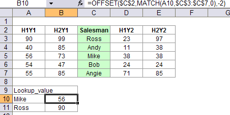
The problem is given in the image sheet below

 

The H1Y1 performance of certain sales people have to be returned. This is achieved through this formula in cell B10

Method 1: Match with Offset

B10 = OFFSET($C$2,MATCH(A10,$C$3:$C$7,0),-2)

This is then dragged to cover all sales people for which figures are required.

Note: match function returns the placement of lookup_value in the column, this is then used to offset. Note that offset reference (C2) is one cell above the lookup column (C3:C7) to ensure that if match returns 1, offset gives a correct value

Method 2: Sum as an array function

B10 {=SUM(($C$3:$C$7=A10)*$A$3:$A$7)}

entered with ctrl+shift+enter

Method 3: Sumproduct

B10=SUMPRODUCT(–($C$3:$C$7=A10),$A$3:$A$7)

May you find this useful!

Read Full Post »

Unraveling a table

Here is the problem that I faced

 

 

 

 

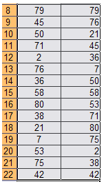
I had to extract the entries in the table row-wise and populate this in a single column.
Here is one way of doing this:

• Enter A8=OFFSET($A$2,INT((ROW()-ROW($B$8))/5),MOD((ROW()-ROW$B$8)),5),1,1)
• Drag down till the entire table is unravelled.

What if we had to unravel the table column wise i.e. in the order A2, A3, A4 etc

Here is the formula that you need to enter in B8 and drag till the last table entry

B8=OFFSET($A$2,MOD((ROW()-ROW($B$8)),3),INT((ROW()-ROW($B$8))/3),1,1)

One could also extract the table in a columnar format. We would have to switch row for column to do so.

mod has the syntax mod(number, divisor) and returns the remainder when number is divided by the divisor. In the above case when the divisor is 3, it returns 0,1,2,01,2 and so on

int(number) returns the nearest integer less than or equal to the number. In the above case int returns 0,0,0,1,1,1,2,2,2 and so on

This is exactly what we need to offset from the reference in the table and unravel it.

Note the divisor in the two formulas, in the first formula the divisor is 5, which is equal to number of columns in the table

In the second formula divisor is 3, which is equal to number of rows in the table

This could also be computed through columns(A2:E4) and rows(A2:E4) respectively

Let me know if you ever find this tip useful or are not clear about any part of the post.

In the meantime, have fun working with excel 🙂

Read Full Post »

Multiple extraction through vlookup

The problem here is extraction of multiple results from a two column array through a vlookup

 

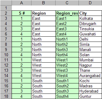
The data available is given in columns B and D. The 4 regions along with their major cities are known. The data needs to be arranged as in the table below

Start by sorting on region (column B)

Column A is populated with serial numbers such that each region has a fresh series

Cell A3=1, Cell A4=IF(B4=B3,A3+1,1) – drag till end of column

Column C is concatenation of columns B and A

Cell C3=CONCATENATE(B3,A3) – drag till end of column

This enables us to have a one on one mapping with region and cities

Now, to generate the result table on the right

Cells – G1:J1 is manually populated with numbers 1 through 4

Cell G2=VLOOKUP(CONCATENATE($F2,G$1),$C$3:$D$18,2,FALSE) – drag till end of column and end of row

’tis done!

Alternative solution 1 using offset

To generate the table in F11:G14

Populate F11 to F14 with East, West, North, South

Here again, we would have to sort on region (column B) first

Enter G11 = IF((COLUMN()-COLUMN($G$1))<COUNTIF($B$3:$B$18,$F11),OFFSET($D$3,MATCH($F11,$B$3:$B$18,0)-1+(COLUMN()-COLUMN($G$1)),0,1,1),””)

Here,

column()-column($G$1) generates numbers 0,1 etc

countif – returns number of occurences of east, west, etc

offset – offsets from the reference cell D3, number of rows given by first occurence of east – provided by match function + serial number given by the column function

You could seperate each of the functions to understand how this works. If you need any help in understanding do let me know

 

Drag to the right and below to populate the entire table

’tis done again

Alternative solution 2 using index

To generate the table in F18:G21

Populate F18 to G21 with East, West, North, South

Enter G18 =IF((COLUMN()-COLUMN($G$1))<COUNTIF($B$3:$B$18,$F11),INDEX($D$3:$D$18,MATCH($F11,$B$3:$B$18,0)+(COLUMN()-COLUMN($G$1))))

Drag to the right and down to populate the entire table.

’tis done once again

Read Full Post »

Reversing order of a table

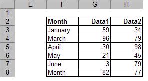
I had saved monthly data by adding months on top of the heap (as in table)

Now while presenting this data, I wanted the data to appear in chronological order, January in row 1, February in row 2 and so on.

 

 

I achieved this by using the offset function.
In cell F3 enter the formula =OFFSET(B$3,8-ROW(),0,1,1)

Drag the formula to the right and down to create a new table.

Here constant 8 is the row number of the last row in the source table. This would work only when the first data row is at the same level as the first data row in the source table (F3 is in the same row as B3)

In practice though if constant is the last row number of the destination table, it would work even when the first rows of source and destination tables are at different level

Read Full Post »