Feeds:
Posts
Comments

Posts Tagged ‘lookup’

lookup_value as array, why lookup over vlookup, multiple lookup_value in single lookup function, sum(lookup)

In one of my earlier posts, I had illustrated passing an array for col_index_num in vlookup. Refer Extract and sum vlookup results.

We now look at the possibility of passing an array for lookup_value in vlookup. Refer the example below:
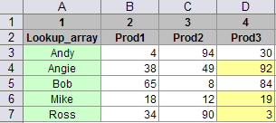
tip30-sum_mult_lookup_value

If we were required to sum the sale of Prod3 for Angie, Mike and Ross (cells highlighted in yellow), can we do it through a single vlookup function. Lets say an array is defined as {Ross, Mike, Angie} as salesperson.

This vlookup function

{=SUM(VLOOKUP(salesperson,A3:D7,4,FALSE))} entered as an array with ctrl+shift+enter gives the result as 3 – which corresponds to sale of Prod3 by Ross (first element in the array salesperson). So clearly the array function is not working!

Lets now try the lookup function. Revise the above formula as

{=SUM(LOOKUP(salesperson,A3:D7))}

OR

{=SUM(LOOKUP(salesperson,A3:A7,D3:D7))}

which depends on your comfort with the two syntax for lookup

  • LOOKUP(lookup_value,array)
  • LOOKUP(lookup_value,lookup_vector,result_vector)

entered as an array formula with ctrl+shift+enter

The formula works and it correctly returns 114

The point to notice here is that lookup_array needs to be in ascending order.

Have fun. This is only the second time that I have used lookup function. It also explains why in the previous post – Text to numbers – method 2, I have used lookup and not vlookup.

Have fun 🙂

Read Full Post »

Just like that, each alphabet corresponds to a number, summing up alphabets

I cant really see how this post could be useful to you. One of my friends who believed in numerology brought this problem to me of converting names to numbers. Here is the solution that we worked out. You may treat this as a Just Like That entry until it finds any use.

Lets say the names are stored in column A, have worked out a numerical equivalent in column B using the equivalence (A or a =1) and (Z or z = 26) with all other alphabets in between

tip29-text_to_numbers

Method 1: Using CODE function

For windows CODE(text) returns the ANSI code of the first character in the text string.

  • code(“A”)=65 and code(“Z”)=90 with all other upper case alphabets in between
  • code(“a”)=97 and code(“z”)=122 with all other lower case alphabets in between

The formula in B2 {=SUM(CODE(MID(LOWER(A2),ROW(INDIRECT(“1:”&LEN(A2))),1))-96)}

entered as an array formula with ctrl+shift+enter

Here lower function is used so that all alphabets are treated as lower case and ansi code is from 97 to 122

Hence, 96 is subtracted so that has numerical equivalent of 1

Cell A4 (Anup Agarwal) has space between the first name and last name. We can use substitute function to replace the space with no space. The revised formula in cell B4 is

B4 {=SUM(CODE(MID(LOWER(SUBSTITUTE(A4,” “,””)),ROW(INDIRECT(“1:”&LEN(SUBSTITUTE(A4,” “,””)))),1))-96)}

again entered as an array formula with ctrl+shift+enter

Method 2: Using lookup function

You can avoid using CODE function and use the lookup function to achieve the same result. Have defined the following table as equivalent

tip29-text_to_numbers_equivalent


The formula entered in B2  {=SUM(LOOKUP(MID(A2,ROW(INDIRECT(“1:”&LEN(A2))),1),equivalent))}

entered as an array formula with ctrl+shift+enter

The formula entered in B4 is

{=SUM(LOOKUP(MID(SUBSTITUTE(A4,” “,””),ROW(INDIRECT(“1:”&LEN(SUBSTITUTE(A4,” “,””)))),1),equivalent))}

entered as an array formula with ctrl+shift+enter

Have fun and let me know if you ever find use of it 🙂

Read Full Post »